

In this tutorial, we will learn how to use Python to perform multiple linear regression. Since we have been introduced to simple linear regression GHOST_URL/how-to-do-simple-linear-regression/. We will use the concepts learned from the article on simple linear regression to build upon it and learn to work with a dataset that is reliant on multiple features to make predictions on the dependent variables. This method is known as multiple linear regression.
For this tutorial, we will be using a publicly available dataset from the UCI machine learning repository. The dataset used is called the Combined Cycle Power Plant and is free to download.
We can start by importing the libraries that will be used to perform this task. These libraries include Pandas, Numpy, Matplotlib, and Scikit-learn.
For this task, we will be importing the LinearRegression module from Scikit-learn to build our model.
import matplotlib.pyplot as plt

%matplotlib inline

import numpy as np

import pandas as pd

from sklearn.model_selection import train_test_split

from sklearn.linear_model import LinearRegression

from sklearn.metrics import r2_score
After importing the necessary libraries, we proceed to load our dataset using Pandas .read_csv function from our working directory.
dataset = pd.read_csv("practice.csv")
We then proceed to view the first five rows in our dataset. This also checks whether the data was read correctly without errors.
dataset.head()
In the cell below we use the .describe() function to give us the statistical information for the dataset. This includes the count, mean, standard deviation, and minimum and maximum values in the dataset.
dataset.describe().transpose()
We then proceed to declare the independent variables X and dependent variables Y from our dataset. In the dataset used AT, V, AP & RH are the independent variables, hence we drop the PE column using the .drop() function. We then store the target column PE in a variable Y.
x = dataset.drop(['PE'], axis = 1).values

y = dataset['PE'].values

print("independent values: ",x)

print("Dependent values: ",y)
We then split the data into training sets and Test sets and placed our variables into the train_test_split() function. The test_size gives the percentage in which we would like to split our dataset, in our case 70% of our data will be split for the training set and 30% split for our test set. We can place our random state to zero so that our results remain the same every time we run our model.
x_train, x_test, y_train, y_test = train_test_split(x, y, test_size = 0.3, random_state = 0)
To train our model, we first initialize our LinearRegression() class and store it in a variable ml. We then use the variable to fit our training data and train our model.
ml = LinearRegression()

ml.fit(x_train, y_train)
Once the model has been trained, we use the .predict function on our test data to generate some outputs.
y_pred = ml.predict(x_test)

print(y_pred)
let's then predict the value of Y from the first rows of the X values using the model we have created and compare the actual result with the predicted result.
ml.predict([[14.96, 41.76, 1024.07, 73.17]])
in the above, the predicted value of our dependent variable "Y" is given from the model
We then evaluate the accuracy of the model using r2_score by comparing the actual test set y_test and the values generated by the model y_pred. This will give us the value of the accuracy of our model.
r2_score(y_test, y_pred)
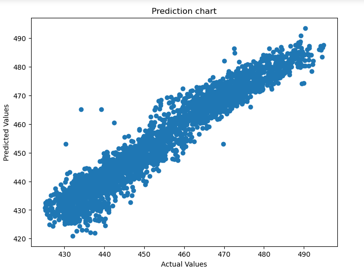
We then visualize the results by using a scatter plot to view the trend of the data. This will give us insight into whether there are outliers.
fig = plt.figure(figsize = (15, 12))

plt.scatter(y_test, y_pred)

plt.xlabel('Actual Values')

plt.ylabel('Predicted Values')

plt.title('Prediction chart')

plt.show()
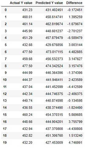
We can also print the predicted Values and compare them to the actual values to see the differences in the two data and judge whether our model needs improvement or is viable.
predicted_y_data = pd.DataFrame({'Actual Y value': y_test, 'Predicted Y value': y_pred, 'Difference': y_test - y_pred})

predicted_y_data[0:20]
Conclusion
In this article, we learn how we can do multiple linear regression. You can also find the code on my GitHub repository https://github.com/IBepyProgrammer/Multiple-Linear-Regression.
If you found this article helpful consider subscribing and sharing.
Thank you.