
In this tutorial, we will learn how to use Python to perform simple linear regression. We will be introduced to dependent variables and independent variables when working with a dataset.
Dependent Variables
Dependent variables, also known as target variables are the variables that you are trying to predict based on the inputs of your model. Simply put these are the outputs from the features of the dataset.
Independent Variables
Independent variables are also known as features/ feature variables. These are the inputs used to make predictions and give the behavior of the target variables. To put it simply we can use the independent variables of the dataset to give us predictions or outputs.
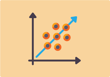
So, what is linear regression?
Linear regression is a form of supervised machine learning that uses a labeled dataset. This means it uses numerical data that is continuous and that may have infinite values.
To give an example data such as length, age, and time can be used in a linear regression where whereas data such as animal species and color would not fit well in a linear regression model as they have a finite category that they can be placed in.
This means that numerical data would be the best fit for linear regression while categorical data would not be a great fit for linear regression.
Build the model
Let's begin by importing the libraries that we will use in the project. The libraries are Pandas, Matplotlib, Numpy, Seaborn, Statsmodels and Sklearn.
Pandas: Pandas is a Python library that will allow us to manipulate, explore, clean, and analyze our dataset.
Matplotlib: Matplotlib is a Python library that allows us to visualize and plot data in the form of graphs, pie charts, and even histograms.
Numpy: Numpy, short for Numerical Python is a library that allows us to work with arrays in Python.
Seaborn: Seaborn library builds upon the matplotlib library as it allows us to make statistical graphs in Python.
Statsmodels: Statsmodels allow us to explore the dataset and extract statistical information from our data.
Sklearn: Sklearn which is short for Scikit-learn is a library that provides us with tools to perform machine learning tasks. These may include model fitting, predictions, cross-validation, and model evaluation.
Note that in the code below we use sklearn.model_selection import train_test_split allows us to split the dataset into training and testing data and also sklearn.metrics import r2_score, mean_squared_error from the Scikit-learn library.
import pandas as pd
import matplotlib.pyplot as plt
%matplotlib inline
import numpy as np
import seaborn as sns
import statsmodels.api as sm
from sklearn.model_selection import train_test_split
from sklearn.metrics import r2_score, mean_squared_error
We will then load our dataset from our working directory or from the directory where the dataset is located using the Pandas library and store it in a variable called dataset.
dataset = pd.read_csv("Book1.csv")
Using the .head() function we can load the first five rows in our dataset. This will also allow us to see whether our dataset was loaded correctly.
dataset.head()
In the cell below we will use the .info() function which gives us information on the dataset such as the number of rows, number of columns, any null values on the dataset as well as the data type we have on the dataset.
dataset.info()
In the next cell, we can use the seaborn library to determine whether there is any correlation between the data in the dataset using a heatmap.
The Correlation value lies between -1.0 and 1.0. The sign indicates whether there is a positive or negative correlation
A -1.0 indicates a perfect negative correlation, whereas +1.0 indicates a perfect positive correlation.
visualization = sns.heatmap(dataset[["Production","Energy Consumption"]].corr(),annot = True)
In the next cell, we Identify the feature X (our independent variable) and outcome Y (our dependent variable) in the dataset to build the model.
From the linear regression formula:
$$ y_i = β_0 +β_1x_i+ε_i $$
Where:
$$ y_i $$ gives the dependent variable.
$$ β_0 $$ gives the population Y-intercept.
$$ β_1 $$ gives the population slope coefficient.
$$ x_i $$ gives the independent variable.
$$ ε_i $$ gives the random error term.
and:
$$ β_0 +β_1x_i $$ is the linear component.
we can build a statsmodels for simple linear regression we will be using the OLS API from the statsmodels library which will help us to estimate the parameters in our linear regression model.
x = sm.add_constant(dataset["Production"])
y = dataset["Energy Consumption"]
print(x.shape)
print(y.shape)
We then split our data into training and test sets. This involves splitting our data into a training set of 80% and our test set into 20%.
x_train, x_test, y_train, y_test = train_test_split(x, y, train_size = 0.80, test_size = 0.2, random_state = 100)
print(x_train.shape)
print(x_test.shape)
print(y_train.shape)
print(y_test.shape)
Note that we could also use from sklearn.linear_model import LinearRegression, to perform linear regression, but for this example, we will be using OLS to fit the model using the training parameters.
data_lm = sm.OLS(y_train, x_train).fit()
Next, we will print the parameters by calling the .params function. This will give us the values for the coefficients and intercepts.
By calling the .summary2() function we get the summarized version of the model.
print(data_lm.params)
data_lm.summary2()
We can then use the model to predict the values of the dataset used. The predicted values can then be further used to measure the accuracy of the model by comparing the predicted values produced by the model from the dataset versus the actual values in the dataset.
#predict values ,Test data set
y_pred_test = data_lm.predict(x_test)
y_pred_train = data_lm.predict(x_train)
To measure the accuracy of our predictions, we will be using the root mean squared error and the $r^2$ which work by taking the predicted values and actual values to calculate the accuracy of the model.
np.abs(r2_score(y_train,y_pred_train))
#np.abs(r2_score(y_test,y_pred_test))
Note that to calculate the root mean squared error method measures the average error the model makes while making the predictions/outcome hence the smaller the value is the better the model.
np.sqrt(mean_squared_error(y_train, y_pred_train))
Once we have measured the accuracy of our predictions, we can move on to visualization of the data. This involves building a scatter plot and drawing a line of best fit between the data points of the scatter plot. This allows us to visualize trends in the data and make predictions. This can also allow us to identify outliers in the data.
plt.figure(figsize = (20,15))
plt.scatter(y_train, y_pred_train, c = 'red')
plt.plot([y_train.min(), y_train.max()], [y_train.min(), y_train.max()],linestyle = 'solid', c = 'green', lw = 3)

plt.xlabel("actual vals")
plt.ylabel("predicted vals")
plt.show()
Conclusion
In this article, we learn how we can do simple linear regression and how to use the different Python libraries to build our model and visualize our predictions. Overall, when you are getting started with machine learning linear regression is a great starter point to get into machine learning models. You can also find the code on my GitHub repository https://github.com/IBepyProgrammer/Simple-Linear-Regression.
If you found this article helpful consider subscribing and sharing.
Thank you.