

In this article, learn how to apply linear regression techniques to solve real-world problems. For this example, you will understand how to perform some simple feature engineering to predict the car prices of vehicles from the dataset provided.
In Jupyter Notebook, import the libraries useful for the project such as Pandas, Matplotlib, and Scikit-learn.
import pandas as pd
import matplotlib.pyplot as plt
from sklearn.linear_model import LinearRegression
from sklearn import metrics
from sklearn.model_selection import train_test_split
The next step is to read the dataset using the .read_csv function from the Pandas library to load the dataset which is in CSV format. The dataset is then stored in the declared variable df.
df = pd.read_csv("car data.csv")
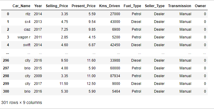
Next, print out the dataset to check whether it has been loaded correctly without errors.
In the dataset, it is visible that there are 301 rows and 9 columns.
df
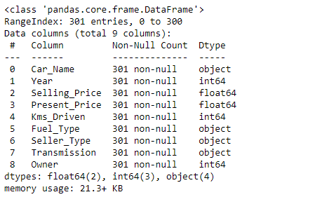
Using the function .info(), information such as the number of rows, number of columns, null values, as well as the data type we have on the dataset is displayed.
This is useful as you can view which columns contain numerical data, categorical data, and even the amount of null values.
Note that with linear regression models, numerical data is what works best and by going through each feature in the dataset we can drop or fill any null values if any are present.
df.info()
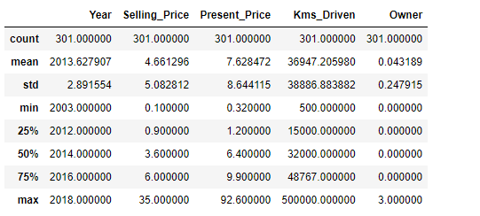
Using the .describe function, the statistical information for the dataset which includes the count, mean, standard deviation, and minimum and maximum values in the dataset is obtained.
df.describe()
In the next step, create a copy of the dataset. This is because, during the process of data analysis, we perform numerous operations on the dataset. This in turn changes the original dataset. A copy of the original dataset is always recommended in case an error occurs. The original dataset can then be referenced at this point.
To then create the copy, use the Pandas copy function and store it in a variable, in this case, df_copy = df.copy(). A copy of the dataset will then be used in the project.
df_copy = df.copy()
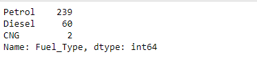
In the next step, proceed to look at each categorical data present. You can look at the value counts and depending on the situation convert the data into numerical data by replacing the objects with integers. This is done as these values may have significance and may impact the performance of the model.
df_copy["Fuel_Type"].value_counts()
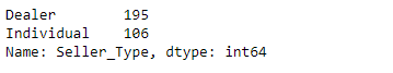
df_copy["Seller_Type"].value_counts()
df_copy["Transmission"].value_counts()
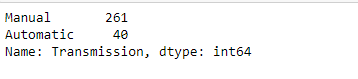
In the outputs above, the column Fuel_Type has petrol and diesel with large values. These can impact the performance and accuracy of the model. This also applies to both the Seller_Type and Transmission columns. These categories can be replaced using integers so that the linear model receives only numerical data.
df_copy.replace({"Fuel_Type":{"Petrol":0, "Diesel":1, "CNG":2}}, inplace=True)
df_copy.replace({"Seller_Type":{"Dealer":0, "Individual":1}}, inplace=True)
df_copy.replace({"Transmission":{"Manual":0, "Automatic":1}}, inplace=True)
After the process of exploring the data, proceed to declare the features and targets from the dataset. In the dataset used, drop the Car_Name and Selling_Price columns using the .drop() function from the features. The next step is to then store the target column Selling_Price in a variable Y.
X = df_copy.drop(["Car_Name", "Selling_Price"], axis=1)
y = df_copy["Selling_Price"]
Split the dataset into training sets and test sets and place the variables into the train_test_split() function from the Scikit-learn library. The test_size, in this case, 80% of the data will be split for training the model and 20% split for testing the model.
X_train, X_test, y_train, y_test = train_test_split(X,y, test_size=0.2, random_state=2)
Training the model will involve initializing the LinearRegression() class and storing it in a variable model. This variable will be used to fit the training data to the machine learning model.
model = LinearRegression()
model.fit(X_train, y_train)
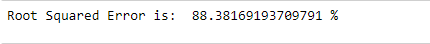
Once the model is trained, you can evaluate the performance accuracy of the training data used. This will show how accurate the model is at reproducing the training data.
train_data_prediction = model.predict(X_train)
error_score = metrics.r2_score(y_train, train_data_prediction)
print("Root Squared Error is: ",error_score*100,"%")
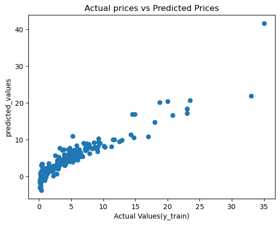
Visualizing the results by using a scatter plot in this case provides a better view of the trend of the data and allows for interaction and understanding of the complex data even better.
plt.scatter(y_train, train_data_prediction)
plt.xlabel("Actual Values(y_train)")
plt.ylabel("predicted_values")
plt.title("Actual prices vs Predicted Prices")
plt.show()
Next, you can evaluate the model's ability to make actual predictions using the testing data.
test_data_prediction = model.predict(X_test)
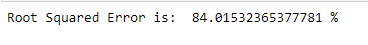
error_score = metrics.r2_score(y_test, test_data_prediction)
print("Root Squared Error is: ",error_score*100,"%")
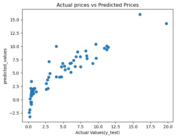
Plot the results of the model prediction with the actual values to view the trend and even find outliers.
plt.scatter(y_test, test_data_prediction)
plt.xlabel("Actual Values(y_test)")
plt.ylabel("predicted_values")
plt.title("Actual prices vs Predicted Prices")
plt.show()
Conclusion
In this article, learn how linear regression builds a model that can be used to predict the prices of cars from a dataset. Overall, the model can always be improved by using different techniques, but in this simple example, we use a simple dataset to understand basic machine learning concepts without much complexity. For references, you can also find the Jupyter Notebook on my GitHub repository https://github.com/IBepyProgrammer/Car-prices-prediction.
If you found this article helpful consider subscribing and sharing.
Thank you.